Brachistochrone curve explained (with some help from Mathcad)

If you wanted to roll a marble down a ramp in the shortest amount of time possible, how would you design that ramp? With a brachistochrone curve.

The Problem

Since childhood we have been told the shortest distance between two points is a straight line. If you are doing that on a sphere, like an airplane, the shortest distance is a great curve. But under the effects of gravity, what is the fastest path to travel between two point?

Johann Bernoulli proposed this challenge to the greatest mathematicians of his day in 1696. Besides himself, five mathematicians responded with solutions, including but not limited to:

• Gottfried Leibniz, one of the founders of calculus.
• Johann’s brother Jakob.
• Sir Isaac Newton, the other founder of calculus, who was more annoyed than challenged. He solved the problem in under twelve hours.

The Solution

Intuition tells us that the more vertical the curve is at the beginning, the more momentum (the product of mass times velocity) the object will gain. Even though it travels a longer distance, it arrives in less time.

Solutions fall into two categories: the direct and indirect method. The former uses a lot of trigonometry and geometry, whereas the latter (which I prefer) incorporates physics.
First, we will use PTC Mathcad to find the time as a function of distance between the points for a straight line. We can convert the ball’s potential energy at the start to kinetic energy at the end.

Initially we will assume that some of the energy gets converted into the rolling motion of a ball.

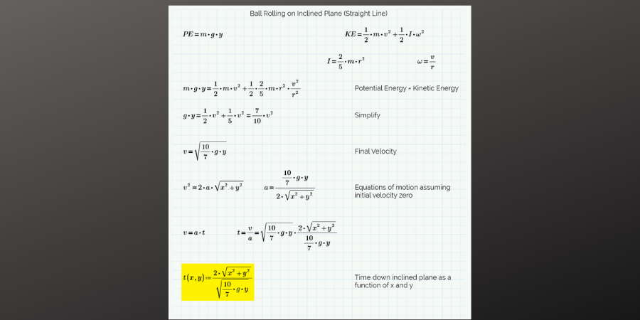
In this solution, I used the following aspects of Mathcad:

• The Comparison operator to walk through the derivation and document equations that are not being solved.
• Text boxes to document the steps.
• Built-in variables for the acceleration due to gravity.
• A function definition that can be used throughout the worksheet.
• Math formatting to draw a person’s attention to the conclusion.

As mentioned earlier, I prefer the indirect approach. (For a great video on the subject, please see the video “The Brachistochrone, with Stephen Strogatz” on the 3Blue1Brown YouTube channel.) Johann Bernoulli solved the problem using:

• Fermat’s principle, also known as the principle of least time, which states that light travels the path that takes the least time.
• Snell’s law, which relates the angle of incidence to the angle of refraction when light passes through different media. (Like when you stick a pencil in a glass of water and the image bends.)

I won’t pretend to understand the derivatives and differential equations in Bernoulli’s solution, but I can document the rest in Mathcad using the Comparison operator:

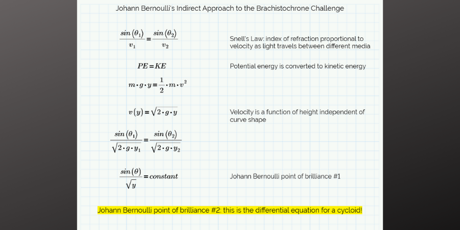
The path is a cycloid: the curve shape when you trace the motion of a point on a circle as it rolls on a straight line. (Aside: mechanisms mode in Creo has a cycloidal motor profile to simulate the motion of a cam.)

Now we will use Mathcad to find the shape of the cycloid that produces the fastest motion between two points.

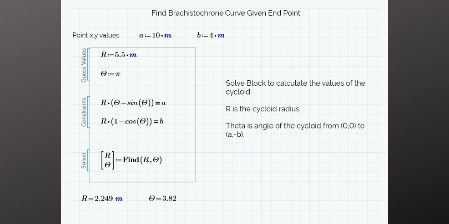
Here I am using the following functionality:

• Mathcad’s inherent understanding of units. As a matter of fact, I found a mistake when the travel times were reported in incorrect units.
• The Solve Block construct with the Find function to solve a system of equations. (the Find function can be found in the function category for Solving)

Now we can compare the travel times between a straight line and a cycloid:

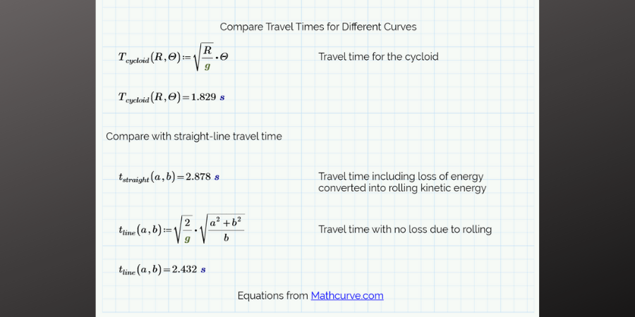
Note the hyperlink in the documentation. This helps others understand the background of the problem.
Mathcad’s Chart Component functionality can plot the path of the cycloid from the start to the end:

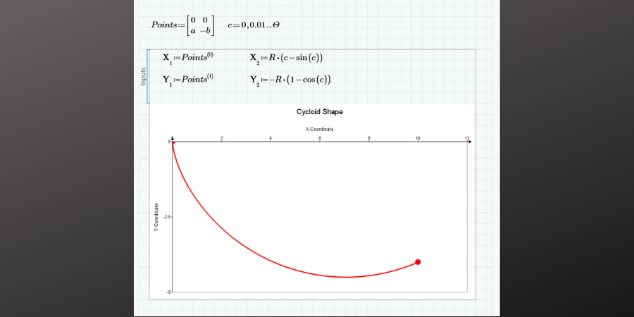
This uses the following Mathcad functionality:

• A matrix to define the start and end points, which are used as one of the plots in the chart (albeit without a line or curve connecting the points).
• A range variable to graph the cycloid.
• Chart formatting including titles, axes labels, custom ranges, and colors.
• Multiple traces/datasets within a plot (one dataset to plot the starting and ending points, and one dataset to plot the curve)

The brachistochrone is an interesting problem from the history of math, and Mathcad has numerous tools to support the investigation.