A general life note: Don’t miss team meetings where tasks are planned and assigned: You’ll invariably get volunteered for something strange. Case in point: I missed the last Mathcad blog-planning session, so I got assigned to write a blog about baseball.
If you knew me well at all, you would understand that I am not a sports person. Don’t get me wrong, I love playing sports, but I just don’t really follow professional or collegiate sports at all. But really, if you have been following the Mathcad blog for very long, you will have probably noticed that our Mathcad and sports correspondent is generally my colleague Tim Bond. He’s explored using math software for better understanding football, golf, and even one for baseball a couple years ago.
In any event, I figure it’s my turn to step up to the plate (side note, for my own personal entertainment, I’m gonna see how many baseball clichés and puns I can sneak in) and swing for the fences (in case you weren’t paying attention, the cliché count is now at two).
But another reason that I may not be the best choice for this post is that I’m from St. Louis, which makes me, by definition, a Cardinals fan. And tragically, the Cardinals are 17 games behind the—I shudder to even mention the name—the Chicago Cu—
Sorry, I passed out from the pain. I’m back now. Let’s just move on from that, shall we?
If I were to write about actually MLB happenings, my lack of knowledge in that arena would make this blog post a swing and a miss. So instead of striking out, I’m going to write about a little program I wrote in Mathcad that computes the trajectory of a baseball, accounting for air resistance. [Ed: Already installed a seat of Mathcad? You can follow along by downloading Luke’s worksheet from the PTC Community.]
Start with Force
As you probably know, a projectile’s trajectory cannot be calculated analytically. You have to perform an infinite number of looped calculations because the force on the ball is directly proportional to the speed of the ball squared.

Force equation, as shown in Mathcad calculation software.
Here, the proportionality constant D is given by

Equation for D.
where, ρ is the air density, A is the cross-sectional area of the ball, and C is the drag coefficient, which is 0.5 for spheres (this is obviously simplified; a baseball, with its texture and seams, would have a slightly different drag coefficient).
Finding Air Density
To find the air density in St. Louis (I’m using Busch Stadium as our location), I used a rather simplified equation that accounts for barometric pressure and temperature, but does not account for humidity. Here is the air density calculation based on the weather conditions in St. Louis at the time of writing this post.
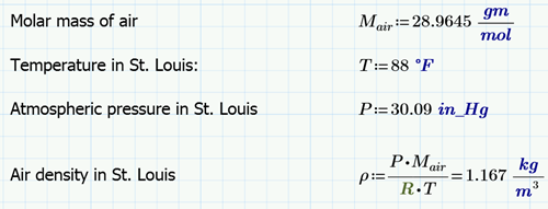
Equations for air pressure variables, as shown in Mathcad calculation software.
Calculating Drag
Using the maximum circumference of 9.25 inches for a baseball, I calculate the maximum cross-sectional area of a baseball, which allows me to calculate the drag proportionality constant for the ball.

Equation for diameter of ball
Finally, I use a baseball mass of 5.25 ounces. With all of this information, I create a function that iterates for the duration of the baseball’s flight, with initial angle, initial position, and initial velocity as the arguments.
How my Mathcad program works
I won’t go through the program step by step, but essentially, it updates the drag force on the baseball and subsequently the x- and y-components of the velocity of the baseball for every hundredth of a second.
The outputs of the program is a 5-row array of arrays, in which the first row is the array of times at which the updates were made, and the other rows are the arrays giving the corresponding x-position, y-position, x-velocity, and y-velocity of the baseball respectively.
The starting x-position of the ball will be zero, and the starting y-position of the ball will be approximated at 3.5 feet. Then, we can choose arbitrary values for angle and initial speed, and plot the trajectory:

Trajectory of ball
Notice the horizontal and vertical markers I added. The horizontal marker shows 8 feet, which is the height of the outfield wall in Busch stadium. The vertical marker shows 400 feet, which is the distance to the outfield wall at center field.
But I wanted to knock this blog out of the park, so I took it a step further and mapped out the baseball field. It’s a bit simplified, since the outfield wall isn’t a consistent 400 feet from home plate, but you get the picture.

St. Louis' Busch Stadium graphed in Mathcad.
The blue x is the pitcher’s mound, the green arc is the grass line, and the brown arc is the (simplified) outfield wall. The red dot is the distance that the baseball travels.
Now, there are certain effects that my model does not account for, such as wind and backspin, but it’s still rather interesting to see an estimate of the baseball’s flight in perspective.
In case you were curious, according to my model, the ball would have to be hit 137 miles per hour to achieve a homerun, assuming an initial angle of trajectory of 37 degrees.
Of course, there is still one question that Mathcad cannot answer: Who is on first?
If you have burning mathematical questions, why not download Mathcad and find the answers for yourself? Mathcad is engineering math software that helps you perform, analyze, and share all your most vital calculations. Engineers at ground-breaking companies use it, and now you can try your own free-for life-version and see what this powerful math software can do for you. Download PTC Mathcad Express today.
