Editor’s note. Guest blogger, Alejandro Rivera, Aerospace Engineer at Goddard Space Flight Center,* returns to discuss the history of Chaos Theory and how Mathcad makes the interpretation and analysis of the Lorenz equations easier.
Chaos theory is a fascinating field of mathematics that studies the behavior of dynamic systems highly sensitive to initial conditions, making their long-term outcome prediction impossible. We live in a complex, dynamic world, and many of the events that surround us are, unbeknownst to us, governed by chaos.
Changes in the weather, varying populations of insects and birds, the rise and fall of civilizations, the expansion of cities, heartbeat irregularities, and even brain activity are all influenced by chaos. Hence, chaos theory has essential applications in engineering, physics, biology, meteorology, sociology, economics, and other disciplines. This article will explore how PTC Mathcad can help analyze even the most complex nonlinear dynamics and chaos problems with relative ease.
Edward Lorenz (1917–2008) was the first to record a known instance of chaotic behavior. As explained by James Gleick in his bestselling book “Chaos – Making a New Science,” Lorenz was a meteorologist at MIT who, in 1955, became the director of a project in statistical weather forecasting. Lorenz had a primitive model of a global weather system that would give approximate predictions. The model used differential equations to capture the relationships among 12 meteorological variables like pressure, temperature, wind speed, etc. The critical component of his model was convection.
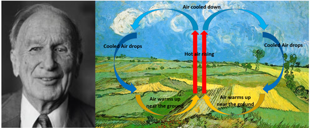
Figure 1: Edward Lorenz and the convection rolls
During convection, the ground heats the air, causing a temperature difference between the lower and higher layers in the atmosphere. When this difference is significant, the lighter, hotter air rises while the cooler air drops. This creates circular convection rolls of air.
In the early days of computing, machines were primarily utilized for complex scientific calculations, and Lorenz was a pioneer in this field. These early computers were primitive, taking up entire rooms and operating at slow speeds. To simplify his weather model, Lorenz decided to make some adjustments. He narrowed it down to three nonlinear differential equations that specifically addressed the convection phenomenon. These equations are commonly referred to as the "Lorenz Equations."
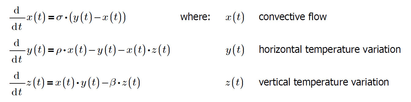
The Prandtl number, represented by σ, indicates the energy loss ratio from fluid viscosity to thermal conduction. The Rayleigh number, represented by ρ, signifies the temperature difference between the top and bottom layers. Meanwhile, the ratio between the height and width of the convective rolls' location is denoted by β.
Lorenz’s computer could handle these equations in a reasonable amount of time. Using different values for the three constants, his computer could calculate how the independent variables changed over time. He then would plot them in the 3D phase space. When he selected σ = 10, ρ = 20, and β = 8/3, he obtained a spectacular trajectory with two distinct interconnected loops resembling a butterfly’s wings.
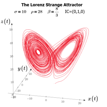
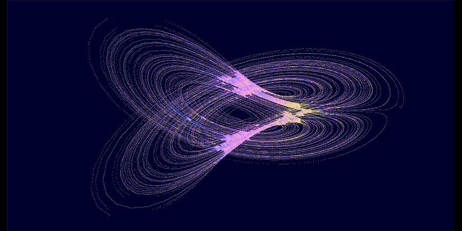
Figure 2: The Lorenz Strange Attractor represented in phase space
Watching the trajectory as it alternates between the left and right wings is mesmerizing. It spends some time on each wing before suddenly switching to the other, repeating this pattern indefinitely without ever crossing over itself. This phenomenon is referred to as the Lorenz Strange Attractor. In nonlinear dynamics, attractors refer to the state that a dynamical system eventually settles into after a certain period. For instance, when a marble is rolled around in a large bowl, it ultimately comes to rest on the bottom. This is because the bottom “attracts” the marble. When dynamical systems never attain this equilibrium, they are known as “strange attractors,” a term coined by David Ruelle in 1970 while explaining the chaotic nature of fluid turbulence.
When we plot the response y(t) in the time domain, we observe that the solution settles into an irregular oscillation as time goes to infinity but never repeats exactly. The motion is nonperiodic.
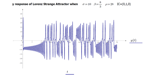
Figure 3: Lorenz attractor and nonperiodic “y response” in the time domain
The story of Lorenz's discovery of chaos is quite captivating. In 1961, while studying a weather prediction sequence, he took a shortcut by starting from the middle of the computer run instead of the beginning. Before taking a coffee break, he entered the numbers from a previous printout directly. Upon his return, he was astounded by the new weather forecast that was vastly different from the original, with two distinct weather systems.
The number he had entered was stored on the printout as 0.506, but the computer’s memory number was 0.506127. Then, he understood what had occurred. A one-part in five thousand difference was not a negligible one. Lorenz immediately understood that even slight variations in the initial conditions, perhaps caused by a small puff of wind, could have far-reaching effects.
Lorenz concluded that this kind of response was built into his model. He published his findings in the Journal of Atmospheric Sciences in a paper titled “Deterministic Nonperiodic Flow” in 1963. Lorenz described the implications of his discovery as follows: “It implies that two states differing by imperceptible amounts may evolve into two considerably different states. If there is an error in observing the present state—and in any real system, such errors seem inevitable—an acceptable prediction of the instantaneous state in the distant future may well be impossible.”
The “Butterfly Effect” is a concept associated with Lorenz. In 1972, he presented a conference paper titled: "Does the flap of a butterfly's wings in Brazil set off a tornado in Texas?" He coined the term to emphasize the immense sensitivity to initial conditions that chaos theory now epitomizes. This extreme sensitivity can be seen in the chart below. If we change y(0 sec) by one millionth while keeping x(0 sec) and z(0 sec) unchanged, the response quickly diverges after roughly 30 seconds. It is no surprise that predicting the weather beyond a few days is a daunting task.
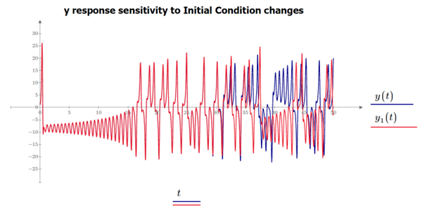
Figure 4: Extreme sensitivity to Initial Conditions of the Lorenz equations in the time domain
Weather forecasting is limited by the amount of information available about a system's parameters, and it's impossible to determine exact initial conditions. As a result, forecasts become less reliable over time and are typically inaccurate beyond a week. The main features of chaos are:
So far, we have presented the basics of chaos and the Lorenz equations. Similar explanations can be found in many books, for example, James Gleick’s. A proper and more thorough understanding of chaos and the Lorenz equations requires analyzing them, and because we are Mathcad users, we have the perfect tool for doing so.
Mathcad Prime makes the interpretation and analysis of the Lorenz equations relatively easy. A Solve Block can be used to solve the Lorenz system of nonlinear differential equations for different initial conditions and parameter values and then plot the responses in phase space.
The mathematical analysis involves studying the local and global stability of the systems’ fixed points and bifurcations for different values of ρ. Before doing so, we must have the right strategy, and a proper mathematical approach is necessary. While we cannot cover the entire mathematical derivation in this article, we will provide some sections of the math to demonstrate Mathcad’s usefulness. Additionally, we will use a graphical approach for the remaining sections.
Let’s start by examining the equations. The Lorenz equations depict a vector field within the 3D phase space. Phase space represents the state of an object in 2D or 3D. It is used to examine dynamic systems as it gives us an overview of the system’s behavior in the form of trajectories that display the system’s evolving state over time corresponding to a specific initial condition. This shows qualities of the system that might not be apparent otherwise.
If we plot a pendulum's angular displacement versus velocity, the resulting trajectory through phase space is a loop (undamped case) or a spiral (damped case). The charts below display the same information: a system that converges to a steady state is displayed as a straight line in the time domain and converges to a point in the phase space plane. Hence, all possible states of the system are conveniently displayed and represented in the phase space.
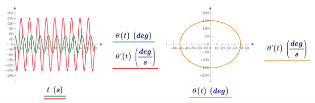
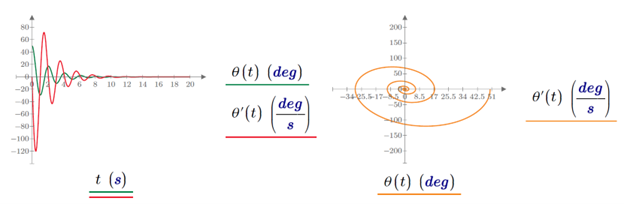
Figure 5: Time domain (left) vs. phase space (right) for an undamped (top) and damped (bottom) pendulum
Going back to the Lorenz system, by inspection, we observe that the system has two nonlinearities: the quadratic terms xy and xz. Also, if we replace (x, y) with (-x, -y), we can see that (-x, -y, z) is a solution, too, so the system is symmetric in (x, y).
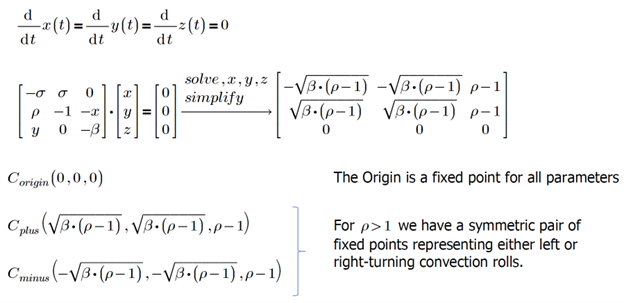
When analyzing dynamic systems, it is critical to understand their fixed points and stability. Within a system of differential equations, the fixed points are those where the first derivatives of the system variables are equal to zero. For example, a pendulum has two fixed points: vertically pointing down under gravity (stable fixed point, also known as attractor) and vertically pointing up (unstable fixed point, also known as repeller). For the Lorenz system, the fixed points are:
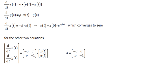
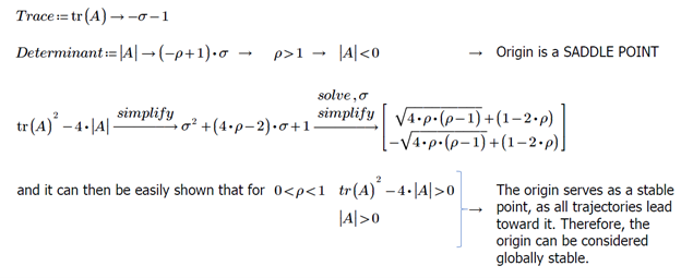
We proceed now to examine the linear Stability of the Origin. We can obtain a decoupled, solvable, linearized version by removing nonlinear terms from the Lorenz equations:
To understand the system’s behavior, we will analyze the Lorenz equations by studying the effect of increasing ρ. The stability of the origin and fixed points are dependent on this parameter. By plotting the Lorenz equations for ρ < 1, we can verify the stability of the origin. For t → ∞, we can observe the convergence of two different trajectories toward the origin.
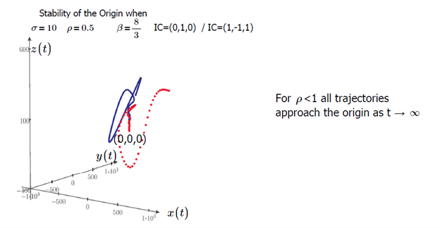
Figure 6: Stability of the Origin in phase space
Let's analyze the linear stability of the remaining fixed points, C+ and C-. As we increase ρ just above one (ρ=1.0005), these fixed points merge with the origin. To confirm this, we can look at a graphical representation.
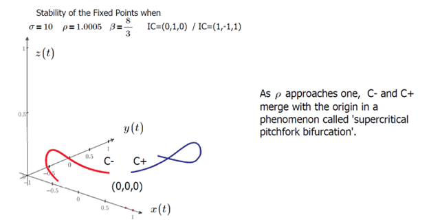
Figure 7: Stability in phase space of the fixed points in the vicinity of ρ=1+
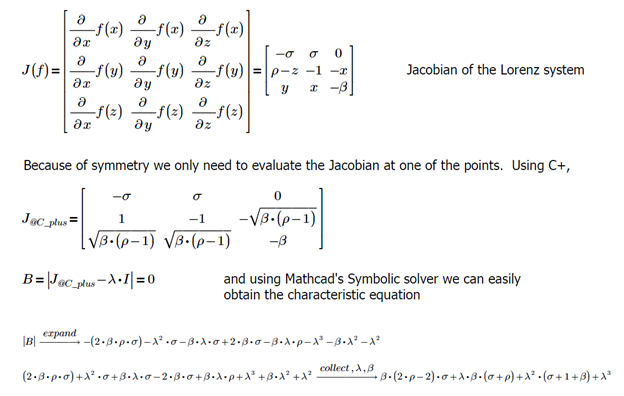
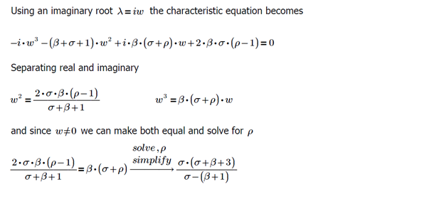
Let's now take a closer look at the fixed points C+ and C- and their stability as ρ increases beyond the value of one. Lorenz's findings confirm that these fixed points do indeed exist. We can learn about their stability by analyzing the characteristic equation of the Jacobian matrix evaluated at one of the fixed points.
Hence, the fixed points C+ and C- are linearly stable for the following range:
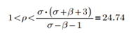
Within this 1<ρ<24.74 interval, there is a homoclinic bifurcation at ρ=13.296. Hence, we will examine the fixed points’ stability for two cases corresponding to 1<ρ<13.926 and 13.926<ρ<24. We can examine the convergence of the trajectories within the 1<ρ<13.926 interval by plotting them for ρ = 5:
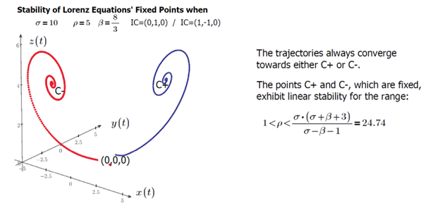
Figure 8: Stability in phase space of the fixed points when 1 < ρ < 13.926 < 24.74
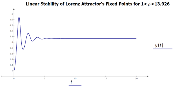
Figure 9: Stability in the time domain of the fixed points when 1 < ρ < 13.926
When the values of ρ fall between 13.926 and 24.08, we refer to it as 'transient chaos.' Figure 10 demonstrates that the trajectories are initially chaotic but ultimately break free and converge towards the C+ or C- fixed points.
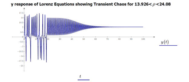
Figure 10: Transient chaos in the time domain when 13.926 < ρ < 24.08
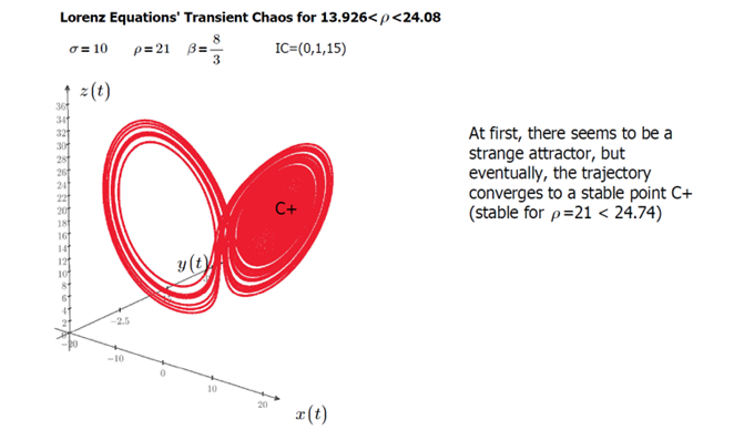
Figure 11: Transient chaos in phase space when 13.926 < ρ < 24.08
As we approach ρ= 24.07, the time spent chaotically moving in the set progressively increases. Finally, at ρ= 24.08, the time becomes infinite, and the set becomes a strange attractor.
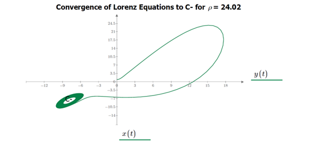
Figure 12: Convergence in phase space to fixed point ‘C-‘ when ρ = 24.02
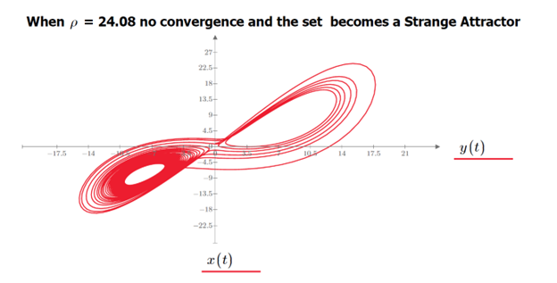
Figure 13: Non-convergence to fixed points when ρ = 24.08 leading to a strange attractor
The interval between 24.08 and 24.74 represents an intriguing phenomenon where both fixed points and a strange attractor can exist simultaneously. For points above 24.74, Lorenz explored the scenario when ρ = 28. After plotting the resulting trajectory using his primitive computer system, he observed how it settled onto an attracting set that resembles a pair of butterfly wings. In this scenario, we no longer have fixed point attractors nearby, requiring trajectories to go to a distant attractor.
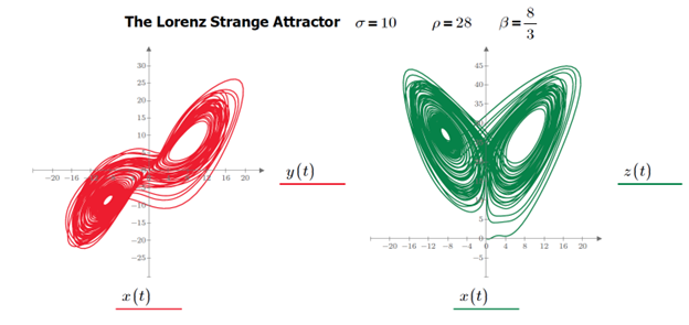
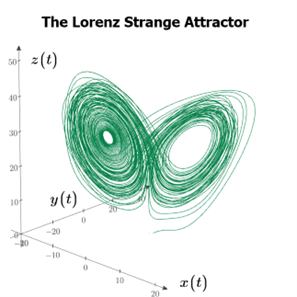
Fig 14: Several views in phase space of the Lorenz strange or chaotic attractor
The strange attractor’s structure consists of two surfaces that blend into each other, giving the impression of a single surface. At the point of merging, there are four surfaces, which then become eight, and so on, creating an infinite number of surfaces that are closely packed together. This complex set of surfaces is known as a fractal, a large collection of points characterized by an infinite surface area but zero volume.
It has been demonstrated that chaos persists between the values of ρ=28 and ρ=313, with occasional small periods of order. However, the system's behavior becomes less complicated for ρ values exceeding 313.
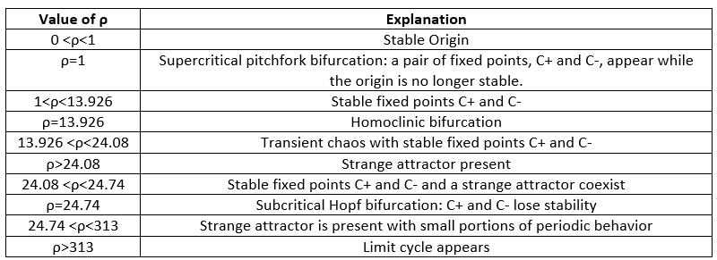
Table 1: Summary of Lorenz equations’ behavior as a function of the parameter ρ
Having gained an understanding of the Lorenz equations, we are now better prepared to revisit the initial atmospheric condition that Lorenz aimed to investigate, which is the dynamic behavior of convection rolls in fluid layers that are heated from below (referred to as rolling fluid convection).
Recall that ρ was the Rayleigh number representing the temperature difference between the bottom and top atmospheric layers. For very low values of the Rayleigh number, there is no significant circulation as the trajectories converge to the origin, which we showed is a globally stable point. However, as the Rayleigh number increases, warmer air rises, and cooler air is displaced and starts to drop, forming circular convection rolls of air. The rotation of the convection cells is steady and converges to the fixed points C+ and C-, which, as shown, are linearly stable.
As the ground warms up and the temperature difference between the top and bottom of the layers increases further, there comes a moment when the Rayleigh number becomes such that the steady convective flow is disrupted, and the trajectories become chaotic. This moment corresponds to the critical Rayleigh number for instability of steady-state convection, which occurs when ρ = 24.74. The back-and-forth changes between the ‘strange attractor wings’ we showed correspond to the changes in the rotation of the convection rolls as the trajectories settle into the chaotic attractor, and a steady state is never reached because the flow becomes turbulent and the convection cells unstable.
Many important lessons can be drawn from Lorenz’s weather model and his discovery of chaos theory. When tackling a complex engineering or scientific problem, a mathematical model can prove extremely useful, allowing us to better understand the physics behind the problem. Mathematical analysis can be difficult, but Mathcad Prime makes it easy. Lorenz would have to wait hours before his primitive computer could integrate his differential equations and produce a solution. Mathcad Prime, however, does it in less than a second. The computational power that we have today, coupled with Mathcad’s ODE solvers for stiff and non-stiff systems, allows us to tackle just about any complex mathematical problem that can be modeled with systems of differential equations. Another essential feature of Mathcad is its symbolic solver, which proves particularly helpful when working with complex algebraic expressions.
It took nearly ten years for researchers to fully understand the importance and consequences of Lorenz's paper on his meteorological model and chaos theory, as these were groundbreaking concepts. Once the scientific community embraced chaos theory, it quickly spread to many fields of science, such as biology, chemistry, engineering, and even economics. Today, chaos theory has even permeated into popular culture, and many books, documentaries, and even movies have used it as inspiration.
In practice, always be on the lookout for chaos when dealing with nonlinear systems with an element of feedback. Chaotic behavior can result whenever nonlinear feedback is present. While Lorenz is popularly recognized as the “father of chaos theory,” it must be mentioned that he was not the first one to encounter it. Almost one hundred years before him, a brilliant French mathematician named Henri Poincaré ran into a chaotic system with nonlinear feedback while trying to solve a problem that had even eluded Isaac Newton. Poincaré showed severe complications when one considered the orbits of three or more gravitating celestial bodies, implying that our solar system was chaotic. We will address this fascinating problem, which in dynamics is known as the 3-body problem, in a future Mathcad article.
[1] Lorenz, E.N., Deterministic nonperiodic flow, Journal of Atmospheric Sciences, 20, 130-141, 1963.
[2] Lorenz, E.N., Predictability: does the flap of a butterfly’s wings in Brazil set off a tornado in Texas? American Association for Advancement of Science, 139th meeting, 1972.
[3] Gleick, J., Chaos - Making a New Science, Penguin Books, 2nd ed., London, 2008.
[4] Lorenz, E.N., The Essence of Chaos, University of Washington Press, 2nd ed, Seattle, WA, 1995.
[5] Rivera, A., Chaos Theory, The Lorenz Equations, and Strange Attractors, Advanced Nonlinear Dynamics Graduate School Project, Washington, DC, 2013.
[6] Williams, R.F., The structure of Lorenz attractors, Publications Mathematiques de l'Institut des Hautes Etudes Scientifiques, volume 50, pages 73-79, 1979.
*The views, methods, and opinions expressed in this article are those of the author and do not necessarily reflect the official policy, procedures, or position of NASA Goddard Space Flight Center or the National Aeronautics and Space Administration. NASA does not promote or endorse any products and this article does not represent an endorsement of Mathcad Prime.
Edward Lorenz photo courtesy of the Lorenz Center at MIT.
Image of “Wheat Fields at Auvers Under Clouded Sky,” by Vincent van Gogh, courtesy of the Carnegie Museum of Art, Pittsburgh, PA.
The author is not affiliated with PTC in any form and received no financial compensation for this article.
Say goodbye to spreadsheets. With Mathcad Prime, you’ll never have to use something else for your engineering or math calculations ever again!